Package Tutorial - Using SVA Correction

Melike Donertas

2019-12-31

Download data and prepare for the analysis

Data is downloaded from GEO using getGEO function in GEOquery library. Expression matrix with probeset IDs, age of the samples and covarietes to be included in the analysis are extracted from geo object. Please note that this tutorial is just to demonstrate the functionality of this package and is not a proper gene expression analysis tutorial. Thus we skip many potential QC steps and probeset -> gene ID mapping.

library(GEOquery)
#> Loading required package: Biobase
#> Loading required package: BiocGenerics
#> Loading required package: parallel
#> 
#> Attaching package: 'BiocGenerics'
#> The following objects are masked from 'package:parallel':
#> 
#>     clusterApply, clusterApplyLB, clusterCall, clusterEvalQ,
#>     clusterExport, clusterMap, parApply, parCapply, parLapply,
#>     parLapplyLB, parRapply, parSapply, parSapplyLB
#> The following objects are masked from 'package:stats':
#> 
#>     IQR, mad, sd, var, xtabs
#> The following objects are masked from 'package:base':
#> 
#>     anyDuplicated, append, as.data.frame, basename, cbind,
#>     colnames, dirname, do.call, duplicated, eval, evalq, Filter,
#>     Find, get, grep, grepl, intersect, is.unsorted, lapply, Map,
#>     mapply, match, mget, order, paste, pmax, pmax.int, pmin,
#>     pmin.int, Position, rank, rbind, Reduce, rownames, sapply,
#>     setdiff, sort, table, tapply, union, unique, unsplit, which,
#>     which.max, which.min
#> Welcome to Bioconductor
#> 
#>     Vignettes contain introductory material; view with
#>     'browseVignettes()'. To cite Bioconductor, see
#>     'citation("Biobase")', and for packages 'citation("pkgname")'.
#> Setting options('download.file.method.GEOquery'='auto')
#> Setting options('GEOquery.inmemory.gpl'=FALSE)
geo <- getGEO('GSE30272',destdir = '~/temp/')[[1]]
#> Found 1 file(s)
#> GSE30272_series_matrix.txt.gz
#> Using locally cached version: ~/temp//GSE30272_series_matrix.txt.gz
#> Parsed with column specification:
#> cols(
#>   .default = col_double(),
#>   ID_REF = col_character()
#> )
#> See spec(...) for full column specifications.
#> Using locally cached version of GPL4611 found here:
#> ~/temp//GPL4611.soft
pd <- pData(geo)
expmat <- exprs(geo)
ages <- setNames(as.numeric(pd$`age:ch1`), pd$geo_accession)
covs <- list(array = as.factor(setNames(pd$`array batch:ch1`, pd$geo_accession)),
bbs = as.factor(setNames(pd$`brain bank source:ch1`, pd$geo_accession)),
sex = as.factor(setNames(pd$`Sex:ch1`, pd$geo_accession)),
race = as.factor(setNames(pd$`race:ch1`, pd$geo_accession)))
ages <- ages[ages >= 20]
expmat <- expmat[, names(ages)]
covs <- lapply(covs, function(x)x[names(ages)])

Calculating the age-related changes in expression level and heterogeneity

We can simply use calc.het function in our package to have all relevant results:

• Here we supply ages in years (‘age_in’ parameter) but we want the model to be constructed on the fourt root scale of age (‘age_to’ parameter).
• We want to apply first SVA and then Quantile Normalisation (‘batch_corr’ parameter) to correct for the confounding factors.
• The age-related change in gene expression will be modelled using a linear model (‘modex’ parameter).
• Data will not be log2 transformed (‘tr_log2’ parameter).
• Features (probesets), will be scaled before the analysis (‘sc_features’ parameter).
• The list of covariates are provided to check the correlation between calculated SVs from unsupervised algorithm SVA.
• We will use spearman correlation coefficient between absolute values of residuals from the model for age-related change in expression level and ages to assess age-related change in expression heterogeneity (‘het_change_met’ parameter).
• All p-values calculated within this function will be corrected for multiple testing using ‘FDR’ (‘padj_met’ parameter).

library(hetAge)
resx <- calc.het(exprmat = expmat[sample(rownames(expmat),1000),], # expression matrix
  age = ages, # age vector
  age_in = 'years',  # scale of the age vector
  age_to = 'pw-0.25', # scale of ages to be used
  batch_corr = 'SVA+QN',  # batch correction method
  modex = 'linear', # model for the change in expression level
  tr_log2 = F, # log2 transform input matrix
  sc_features = T, # scale genes / probesets
  covariates = covs, # covariates
  het_change_met = 'spearman', # method to measure change in heterogeneity
  padj_met = 'fdr') # multiple test correction method
#> Number of significant surrogate variables is:  15 
#> Iteration (out of 5 ):1  2  3  4  5

Result object

The resulting object is a list with several fields.

The list of sampels used in the analysis:

head(resx$sampleID)
#> [1] "GSM750020" "GSM750021" "GSM750022" "GSM750023" "GSM750024" "GSM750025"

The expression matrix inputted in the first place, only including the samples used in the analysis.

resx$input_expr[1:5,1:5]
#>                      GSM750020   GSM750021   GSM750022 GSM750023
#> HEEBO-052-HCC52F4   0.10049472 -0.05629888  0.48009140 0.7026872
#> HEEBO-055-HCC55M14 -0.04526109 -0.13370321  0.18454854 0.1686122
#> HEEBO-062-HCC62C12  0.18587892 -0.22945709  0.75308331 0.2992347
#> HEEBO-058-HCC58H16  0.35549359 -0.18573769 -0.03304151 0.2351208
#> HEEBO-018-HCC18G15  0.27837650  1.04788814  0.49108739 1.0070288
#>                      GSM750024
#> HEEBO-052-HCC52F4  -2.49810601
#> HEEBO-055-HCC55M14 -0.68181162
#> HEEBO-062-HCC62C12  0.61039147
#> HEEBO-058-HCC58H16  0.09478959
#> HEEBO-018-HCC18G15  0.49569428

The ages in the original format, including only the samples used in the analysis

head(resx$input_age)
#> GSM750020 GSM750021 GSM750022 GSM750023 GSM750024 GSM750025 
#>  20.22192  20.78630  20.86301  20.94521  21.01918  21.47397

The ages after re-formetted into desired format

Here we wanted the ages to be in fourth root scale.

head(resx$usedAge)
#> GSM750020 GSM750021 GSM750022 GSM750023 GSM750024 GSM750025 
#>  9.268913  9.332920  9.341518  9.350705  9.358950  9.409170

library(tidyverse)
#> ── Attaching packages ───────────────────────────────────────────────────────────────── tidyverse 1.2.1 ──
#> ✔ ggplot2 3.2.1     ✔ purrr   0.3.2
#> ✔ tibble  2.1.3     ✔ dplyr   0.8.3
#> ✔ tidyr   0.8.3     ✔ stringr 1.4.0
#> ✔ readr   1.3.1     ✔ forcats 0.4.0
#> ── Conflicts ──────────────────────────────────────────────────────────────────── tidyverse_conflicts() ──
#> ✖ dplyr::combine()    masks Biobase::combine(), BiocGenerics::combine()
#> ✖ dplyr::filter()     masks stats::filter()
#> ✖ dplyr::lag()        masks stats::lag()
#> ✖ ggplot2::Position() masks BiocGenerics::Position(), base::Position()
data.frame(age = resx$input_age, age0.25 = resx$usedAge) %>%
  ggplot(aes(x = age, y = age0.25)) +
  geom_point() +
  geom_smooth( method = 'loess') +
  theme_bw()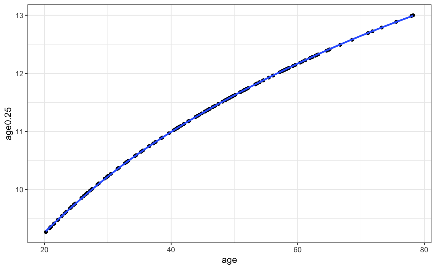

Expression matrix after correcting for confounding factors

These are the expression values for the probesets after accounting for the predicting confounding factors, i.e. SVs

resx$sva_res$correctedExp[1:5,1:5]
#>                      GSM750020   GSM750021   GSM750022    GSM750023
#> HEEBO-052-HCC52F4  -0.06578511  0.21534929  0.14186783  0.177822545
#> HEEBO-055-HCC55M14 -0.34298413 -0.09787721 -0.15968076  0.162312423
#> HEEBO-062-HCC62C12  0.09462668 -0.42847839  0.15059911 -0.009947639
#> HEEBO-058-HCC58H16  0.13975540  0.07335882 -0.10368628  0.188370170
#> HEEBO-018-HCC18G15 -0.11578613  0.32491123 -0.06006239  0.182779324
#>                      GSM750024
#> HEEBO-052-HCC52F4   0.12272472
#> HEEBO-055-HCC55M14 -0.31357715
#> HEEBO-062-HCC62C12  0.31779393
#> HEEBO-058-HCC58H16 -0.08316992
#> HEEBO-018-HCC18G15 -0.04886080

SVs predicted by SVA

head(resx$sva_res$SVs)
#>                  SV_1         SV_2          SV_3         SV_4        SV_5
#> GSM750020 -0.03587305 -0.024489636  0.0059878164 -0.048965239  0.18616121
#> GSM750021  0.02026107  0.107982425 -0.0700008411 -0.036937548 -0.06223375
#> GSM750022 -0.03354348  0.099567309  0.1385842685  0.054784696  0.02114598
#> GSM750023 -0.03361290 -0.068216831 -0.0657148298 -0.004427889 -0.05263926
#> GSM750024  0.10156756 -0.009597882  0.0006723872 -0.080898990 -0.19914128
#> GSM750025 -0.03548707  0.010292602 -0.0397513723 -0.017186732  0.11495601
#>                  SV_6        SV_7         SV_8         SV_9         SV_10
#> GSM750020 -0.02325587 0.002625619 -0.010878374  0.082096963 -0.0007672591
#> GSM750021  0.05018446 0.077027469 -0.042900822 -0.011518120 -0.0904105784
#> GSM750022  0.01499163 0.015735664  0.034467558  0.003291519 -0.0471430470
#> GSM750023  0.02363668 0.097666904 -0.047520740 -0.062625526  0.0811304600
#> GSM750024  0.04171068 0.013182832  0.009590188 -0.004079491  0.0568044997
#> GSM750025 -0.01146978 0.032153027 -0.016301063 -0.030611552  0.0060429281
#>                 SV_11         SV_12        SV_13        SV_14        SV_15
#> GSM750020  0.02490492 -0.0069757346  0.041085093 -0.002524479  0.110370167
#> GSM750021 -0.11006230 -0.0175079243  0.042235402 -0.031401602 -0.002061871
#> GSM750022  0.08235624  0.0303450060 -0.004128296  0.029456621  0.044021529
#> GSM750023 -0.01577012 -0.0003788446  0.201223522  0.030454966 -0.013064804
#> GSM750024 -0.06878366 -0.0157805016 -0.200155145 -0.164437212  0.177333153
#> GSM750025 -0.12081924  0.0105574386 -0.006450429  0.121553328 -0.023115053

Correlation between known potential confounders and predicted SVs

head(resx$sva_res$SV_cov_corr) %>%
  knitr::kable()

cov	estimate	p	p.adj	SV
array.1	0.0196222	0.5814825	0.9353713	1
array.10	0.0225531	0.5265514	0.9353713	1
array.11	0.0834974	0.0231217	0.1695593	1
array.12	0.0332366	0.4305371	0.9353713	1
array.13	0.1496421	0.0000623	0.0013710	1
array.14	0.0576888	0.2368201	0.8872256	1

The expression level matrix used for modeling

This is the matrix used to model age-related expression change - the reason it is different from corrected matrix is because we may further scale the expression level for the features (‘sc_features’ parameter.)

resx$usedMat[1:5,1:5]
#>                     GSM750020  GSM750021  GSM750022  GSM750023  GSM750024
#> HEEBO-052-HCC52F4  -0.4322146  1.1458254  0.8943767 0.93934762  0.6416444
#> HEEBO-055-HCC55M14 -1.9471385 -0.4307714 -1.1183638 0.88710546 -1.4763938
#> HEEBO-062-HCC62C12  0.3279681 -1.5542646  0.7426880 0.01220373  1.2090983
#> HEEBO-058-HCC58H16  0.7429342  0.4505388 -0.8675669 1.22556507 -0.5059969
#> HEEBO-018-HCC18G15 -0.4841314  1.2417387 -0.2949549 0.71294329 -0.1818230

Residuals from the model between expression level and age

Absolute values of this matrix can be considered as the level of heterogeneity for each gene, each sample.

resx$residMat[1:5,1:5]
#>                     GSM750020   GSM750021  GSM750022 GSM750023  GSM750024
#> HEEBO-052-HCC52F4  -0.3897952  1.18682843  0.9351895 0.9799571  0.6820715
#> HEEBO-055-HCC55M14 -1.9324787 -0.41660108 -1.1042593 0.9011398 -1.4624225
#> HEEBO-062-HCC62C12  0.4771780 -1.41003664  0.8862466 0.1550473  1.3513001
#> HEEBO-058-HCC58H16  0.2534892 -0.02256408 -1.3384743 0.7570032 -0.9724537
#> HEEBO-018-HCC18G15 -0.4992009  1.22717231 -0.3094537 0.6985167 -0.1961847

Data frame with the summaries of age-related changes in expression level and heterogeneity

colnames(resx$feature_result)
#> [1] "feature"                    "level_change"              
#> [3] "level_change.p"             "heterogeneity_change"      
#> [5] "heterogeneity_change.p"     "level_change.p.adj"        
#> [7] "heterogeneity_change.p.adj"
head(resx$feature_result) 
#> # A tibble: 6 x 7
#>   feature level_change level_change.p heterogeneity_c… heterogeneity_c…
#>   <chr>          <dbl>          <dbl>            <dbl>            <dbl>
#> 1 HEEBO-…      0.0221        0.799              0.107           0.194  
#> 2 HEEBO-…      0.00765       0.930             -0.225           0.00607
#> 3 HEEBO-…      0.0778        0.370             -0.116           0.160  
#> 4 HEEBO-…     -0.255         0.00285           -0.0786          0.342  
#> 5 HEEBO-…     -0.00786       0.928             -0.115           0.166  
#> 6 HEEBO-…      0.296         0.000512           0.0615          0.458  
#> # … with 2 more variables: level_change.p.adj <dbl>,
#> #   heterogeneity_change.p.adj <dbl>

Session Info

options(width = 100)
sessioninfo::session_info()
#> ─ Session info ───────────────────────────────────────────────────────────────────────────────────
#>  setting  value                       
#>  version  R version 3.6.1 (2019-07-05)
#>  os       macOS Catalina 10.15.2      
#>  system   x86_64, darwin15.6.0        
#>  ui       X11                         
#>  language (EN)                        
#>  collate  en_GB.UTF-8                 
#>  ctype    en_GB.UTF-8                 
#>  tz       Europe/Istanbul             
#>  date     2019-12-31                  
#> 
#> ─ Packages ───────────────────────────────────────────────────────────────────────────────────────
#>  package        * version   date       lib source        
#>  annotate         1.62.0    2019-05-02 [2] Bioconductor  
#>  AnnotationDbi    1.46.0    2019-05-02 [2] Bioconductor  
#>  assertthat       0.2.1     2019-03-21 [2] CRAN (R 3.6.0)
#>  backports        1.1.5     2019-10-02 [2] CRAN (R 3.6.0)
#>  Biobase        * 2.44.0    2019-05-02 [2] Bioconductor  
#>  BiocGenerics   * 0.30.0    2019-05-02 [2] Bioconductor  
#>  BiocParallel     1.18.1    2019-08-06 [2] Bioconductor  
#>  bit              1.1-14    2018-05-29 [2] CRAN (R 3.6.0)
#>  bit64            0.9-7     2017-05-08 [2] CRAN (R 3.6.0)
#>  bitops           1.0-6     2013-08-17 [2] CRAN (R 3.6.0)
#>  blob             1.2.0     2019-07-09 [2] CRAN (R 3.6.0)
#>  broom            0.5.2     2019-04-07 [2] CRAN (R 3.6.0)
#>  cellranger       1.1.0     2016-07-27 [2] CRAN (R 3.6.0)
#>  cli              1.1.0     2019-03-19 [2] CRAN (R 3.6.0)
#>  colorspace       1.4-1     2019-03-18 [2] CRAN (R 3.6.0)
#>  crayon           1.3.4     2017-09-16 [2] CRAN (R 3.6.0)
#>  curl             4.0       2019-07-22 [2] CRAN (R 3.6.0)
#>  DBI              1.0.0     2018-05-02 [2] CRAN (R 3.6.0)
#>  desc             1.2.0     2018-05-01 [2] CRAN (R 3.6.0)
#>  digest           0.6.21    2019-09-20 [2] CRAN (R 3.6.0)
#>  dplyr          * 0.8.3     2019-07-04 [2] CRAN (R 3.6.0)
#>  evaluate         0.14      2019-05-28 [2] CRAN (R 3.6.0)
#>  fansi            0.4.0     2018-10-05 [2] CRAN (R 3.6.0)
#>  forcats        * 0.4.0     2019-02-17 [2] CRAN (R 3.6.0)
#>  fs               1.3.1     2019-05-06 [2] CRAN (R 3.6.0)
#>  genefilter       1.66.0    2019-05-02 [2] Bioconductor  
#>  generics         0.0.2     2018-11-29 [2] CRAN (R 3.6.0)
#>  GEOquery       * 2.52.0    2019-05-02 [2] Bioconductor  
#>  ggplot2        * 3.2.1     2019-08-10 [2] CRAN (R 3.6.0)
#>  glue             1.3.1     2019-03-12 [2] CRAN (R 3.6.0)
#>  gtable           0.3.0     2019-03-25 [2] CRAN (R 3.6.0)
#>  haven            2.1.1     2019-07-04 [2] CRAN (R 3.6.0)
#>  hetAge         * 0.1.0     2019-12-30 [1] local         
#>  highr            0.8       2019-03-20 [2] CRAN (R 3.6.0)
#>  hms              0.5.0     2019-07-09 [2] CRAN (R 3.6.0)
#>  htmltools        0.3.6     2017-04-28 [2] CRAN (R 3.6.0)
#>  httr             1.4.1     2019-08-05 [2] CRAN (R 3.6.0)
#>  IRanges          2.18.1    2019-05-31 [2] Bioconductor  
#>  jsonlite         1.6       2018-12-07 [2] CRAN (R 3.6.0)
#>  knitr            1.24      2019-08-08 [2] CRAN (R 3.6.0)
#>  labeling         0.3       2014-08-23 [2] CRAN (R 3.6.0)
#>  lattice          0.20-38   2018-11-04 [2] CRAN (R 3.6.1)
#>  lazyeval         0.2.2     2019-03-15 [2] CRAN (R 3.6.0)
#>  limma            3.40.6    2019-07-26 [2] Bioconductor  
#>  lubridate        1.7.4     2018-04-11 [2] CRAN (R 3.6.0)
#>  magrittr         1.5       2014-11-22 [2] CRAN (R 3.6.0)
#>  MASS             7.3-51.4  2019-03-31 [2] CRAN (R 3.6.1)
#>  Matrix           1.2-17    2019-03-22 [2] CRAN (R 3.6.1)
#>  matrixStats      0.54.0    2018-07-23 [2] CRAN (R 3.6.0)
#>  memoise          1.1.0     2017-04-21 [2] CRAN (R 3.6.0)
#>  mgcv             1.8-28    2019-03-21 [2] CRAN (R 3.6.1)
#>  modelr           0.1.5     2019-08-08 [2] CRAN (R 3.6.0)
#>  munsell          0.5.0     2018-06-12 [2] CRAN (R 3.6.0)
#>  nlme             3.1-140   2019-05-12 [2] CRAN (R 3.6.1)
#>  pillar           1.4.2     2019-06-29 [2] CRAN (R 3.6.0)
#>  pkgconfig        2.0.3     2019-09-22 [2] CRAN (R 3.6.0)
#>  pkgdown          1.4.1     2019-09-15 [2] CRAN (R 3.6.0)
#>  plyr             1.8.4     2016-06-08 [2] CRAN (R 3.6.0)
#>  preprocessCore   1.46.0    2019-05-02 [2] Bioconductor  
#>  purrr          * 0.3.2     2019-03-15 [2] CRAN (R 3.6.0)
#>  R6               2.4.0     2019-02-14 [2] CRAN (R 3.6.0)
#>  Rcpp             1.0.2     2019-07-25 [2] CRAN (R 3.6.0)
#>  RCurl            1.95-4.12 2019-03-04 [2] CRAN (R 3.6.0)
#>  readr          * 1.3.1     2018-12-21 [2] CRAN (R 3.6.0)
#>  readxl           1.3.1     2019-03-13 [2] CRAN (R 3.6.0)
#>  reshape2         1.4.3     2017-12-11 [2] CRAN (R 3.6.0)
#>  rlang            0.4.0     2019-06-25 [2] CRAN (R 3.6.0)
#>  rmarkdown        1.14      2019-07-12 [2] CRAN (R 3.6.0)
#>  rprojroot        1.3-2     2018-01-03 [2] CRAN (R 3.6.0)
#>  RSQLite          2.1.2     2019-07-24 [2] CRAN (R 3.6.0)
#>  rstudioapi       0.10      2019-03-19 [2] CRAN (R 3.6.0)
#>  rvest            0.3.4     2019-05-15 [2] CRAN (R 3.6.0)
#>  S4Vectors        0.22.0    2019-05-02 [2] Bioconductor  
#>  scales           1.0.0     2018-08-09 [2] CRAN (R 3.6.0)
#>  sessioninfo      1.1.1     2018-11-05 [2] CRAN (R 3.6.0)
#>  stringi          1.4.3     2019-03-12 [2] CRAN (R 3.6.0)
#>  stringr        * 1.4.0     2019-02-10 [2] CRAN (R 3.6.0)
#>  survival         2.44-1.1  2019-04-01 [2] CRAN (R 3.6.1)
#>  sva              3.32.1    2019-05-22 [2] Bioconductor  
#>  tibble         * 2.1.3     2019-06-06 [2] CRAN (R 3.6.0)
#>  tidyr          * 0.8.3     2019-03-01 [2] CRAN (R 3.6.0)
#>  tidyselect       0.2.5     2018-10-11 [2] CRAN (R 3.6.0)
#>  tidyverse      * 1.2.1     2017-11-14 [2] CRAN (R 3.6.0)
#>  utf8             1.1.4     2018-05-24 [2] CRAN (R 3.6.0)
#>  vctrs            0.2.0     2019-07-05 [2] CRAN (R 3.6.0)
#>  withr            2.1.2     2018-03-15 [2] CRAN (R 3.6.0)
#>  xfun             0.8       2019-06-25 [2] CRAN (R 3.6.0)
#>  XML              3.98-1.20 2019-06-06 [2] CRAN (R 3.6.0)
#>  xml2             1.2.2     2019-08-09 [2] CRAN (R 3.6.0)
#>  xtable           1.8-4     2019-04-21 [2] CRAN (R 3.6.0)
#>  yaml             2.2.0     2018-07-25 [2] CRAN (R 3.6.0)
#>  zeallot          0.1.0     2018-01-28 [2] CRAN (R 3.6.0)
#> 
#> [1] /private/var/folders/z1/nv26gvmx4_11_968lfd0n5rh0000gn/T/RtmpAH4Avp/temp_libpath729350b707e8
#> [2] /Library/Frameworks/R.framework/Versions/3.6/Resources/library