Bölüm 6 Temel bilesenler analizi

tba = prcomp(t(genexpr_qn), scale. = T)

renkler = colorRampPalette(c('pink','darkred'))(length(yas))
renkler_sirali = renkler[rank(yas[rownames(tba$x)], ties.method = 'min')]
plot(x = tba$x[,1], y = tba$x[,2], pch = 19, cex = 0.5, col = renkler_sirali, 
     xlab = 'PC1', ylab = 'PC2')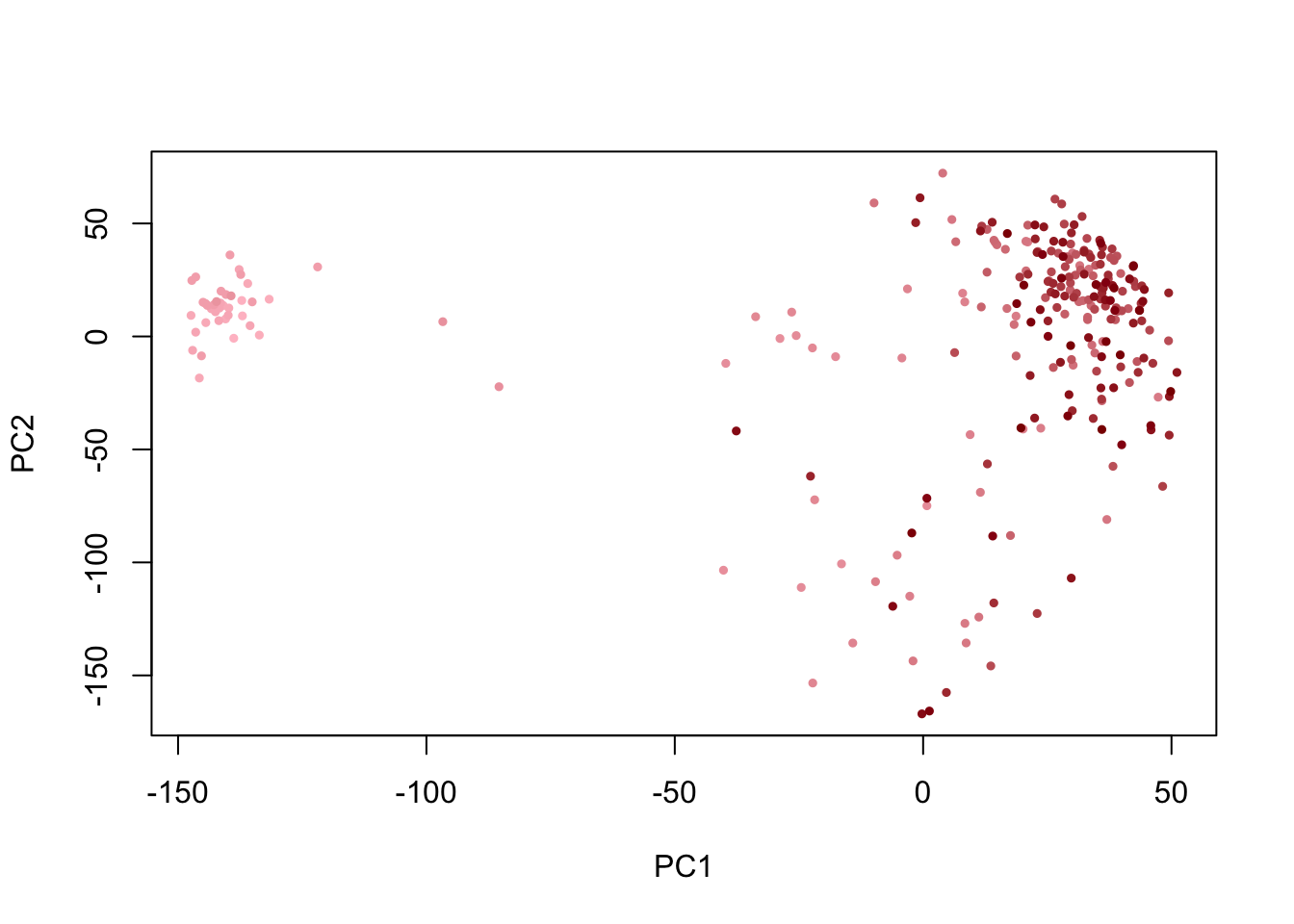

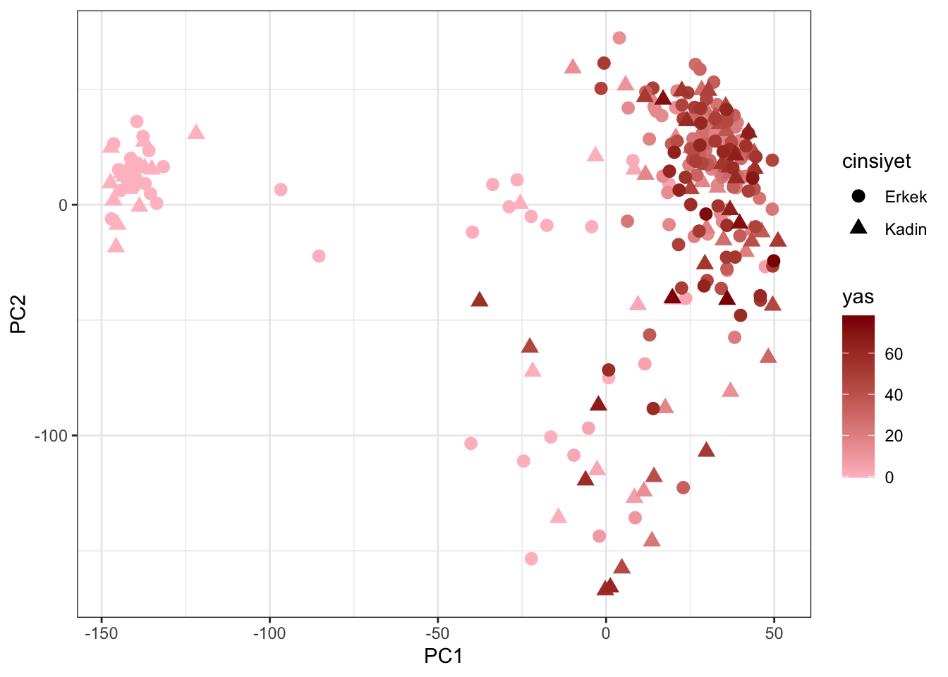
Ayni figuru ggplot ile yapabiliriz. Ancak bunun icin bir kac tidyversede yer alan paketlerden bir kac fonksiyon kullanarak veriyi sekillendirmem gerekiyor:

library(tidyverse)

## ── Attaching packages ─────────────────────────────────────── tidyverse 1.3.0 ──

## ✓ tibble  3.0.6     ✓ dplyr   1.0.2
## ✓ tidyr   1.1.0     ✓ stringr 1.4.0
## ✓ readr   1.3.1     ✓ forcats 0.5.1
## ✓ purrr   0.3.4

## ── Conflicts ────────────────────────────────────────── tidyverse_conflicts() ──
## x dplyr::filter() masks stats::filter()
## x dplyr::lag()    masks stats::lag()

pcadat = as.data.frame(tba$x[,1:2]) %>%
  mutate(sample = rownames(tba$x)) %>%
  mutate(yas = yas[sample],
         cinsiyet = cinsiyet[sample])
head(pcadat)

##         PC1        PC2    sample        yas cinsiyet
## 1 -138.7854 -0.7978871 GSM749899 -0.4986301    Kadin
## 2 -137.1751 15.9124596 GSM749900 -0.4986301    Kadin
## 3 -142.7689 13.8844269 GSM749901 -0.4986301    Erkek
## 4 -137.0419  9.0980053 GSM749902 -0.4986301    Erkek
## 5 -133.6389  0.6007799 GSM749903 -0.4794521    Erkek
## 6 -131.6583 16.4774424 GSM749904 -0.4794521    Erkek

ggplot(pcadat, aes(x = PC1, y = PC2, color = yas, shape = cinsiyet)) +
  geom_point(size = 3) +
  scale_color_gradient(low = 'pink', high = 'darkred') +
  theme_bw()